PyDepth Project
Skip to the interesting sections!
Introduction
What we did
Materials and Methods
How we did it
Results: Method 1
What we got
PyDepth is a student-led project aimed at creating depth maps from stereo images. Throughout this project two methods were explored, both of which used convolutional neural networks and were grounded in machine learning.
With autonomous devices becoming more widely used, there is a need for implementation of object-avoidance systems within these devices. This can be achieved by creating depth maps of the environment.
Deep Convolutional Neural Networks are powerful machine learning algorithms that can be put to use in various circumstances. PyDepth is a student led project in which Convolutional Neural Networks are used in an attempt to create 3D models of an environment. Similarly to human eyes, the project strives to create an accurate evaluation of depth from two images taken by a stereo camera. Two methods are tested and explored: The first method fully relies on the learning capabilities of neural networks. The left and right images generated by the stereo camera are fed through a Dual input Convolutional Neural Network, and the network is trained to generate depth maps using prebuilt maps. The second method constructs disparity maps using the parallax shift between the left and right stereo images. It uses a Dual input Convolutional Neural Network to identify the parallax shift for each pixel and an iterative programme to generate the depth maps. Whilst the results of this study do indicate that generating depth maps with these two methods might be possible, it is clear that much optimisation would be needed to implement them accurately and in real time.
What we did
How we did it
What we got
Why we got it
What we think about what we got
Who did what
Introduction and Theory
PyDepth is a continuation of a previous student-led project, PyStalk, in which an algorithm was built and implemented in a drone to detect and track individuals. It was observed that whilst the tracking was correctly implemented, the drone was unable to circumvent objects placed in its path. Object detection and obstacle avoidance have the potential to increase the effectiveness of autonomous surveillance drones and to handle object-avoidance issues. This project is aimed at introducing two ways of implementing object avoidance through the use of depth and disparity maps of the surroundings. This was achieved by using Dual input Convolutional Neural Networks (DiCNN) at the core of each method.
Artificial Neural Networks
Essential parts of this project were computational algorithms used to attain depth perception maps. Artificial Neural Networks (NN) are a set of algorithms modeled on the human brain, which have been shown to be efficient for machine learning (Haykin, 2009). They generally consist of three main sections: an input layer, one or more hidden layers, and an output layer. Each layer plays an essential role and is comprised of a set of nodes, connected to one another via weights (see Figure 1). Using this structure, the algorithms can be trained to recognise patterns in datasets.
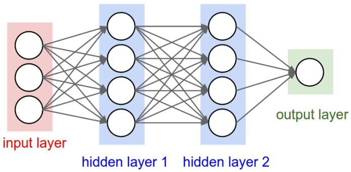
Figure 1: Illustration of the structure of a Neural Network with its three main sections: an input layer, hidden layers and an output layer. Each node is represented by a white circle and each weight by a connecting line (Fonau et al., 2019).
In the context of this project, the input layer receives the pixel values of the images. Each Red-Green-Blue (RGB) image consists of three tensors (one for each colour) of numbers between 0 and 255. This scale gives the brightness of each colour channel within that pixel. To feed these values through an NN, they all get flattened into a one dimensional tensor and each value gets assigned to a node. Each node is connected to all the nodes in the adjacent layer (one of the hidden layers) by a set of numbers called weights. The values that are assigned to each of the nodes (except the input layer) are given by the following formula:
CurrentNode = Σ_i (PreviousNode)_i * Weight_i
After each layer there is an activation function. Activation functions convert input signals of a node into a well defined output. The function evaluates the relevance of a node and determines whether it should be active or not. These functions are essential for NN to learn and make sense of complicated data. There are many activation functions with different properties. One of the most widespread functions and also the one used in this project is the Rectified linear Unit (ReLu). Much like a half wave rectifier in electronics engineering, it is defined as the positive part of an argument:
f(x) = max(0,x)
Additional concepts relative to NNs are supervised learning and backpropagation. Supervised learning is a method in which a NN learns to find patterns in data with already known outputs. A NN is given a set of data and gives an arbitrary output, which is then compared to the desired output of that data. Depending on how far off the NN is, it will adjust its weights to best match the desired output. This process is called backpropagation. In repeating backpropagation multiple times, the NN trains and eventually the NN should be able to predict desired outputs from previously unseen data (Hecht-Nielsen, 1992).
Lastly, NNs often have an additional parameter called bias. A bias is a value that is added across different nodes. It is used as a constant that helps the network best fit the given data and for ensuring that certain layers do not go to zero (Lawrence et al, 1996).
Convolutional Neural Networks
A Convolutional Neural Network (CNN) is a class of deep NNs often used in visual imagery analysis. What distinguishes them from classical NNs is the addition of convolutional layers. In the case of imagery analysis, a convolutional layer is a NN layer that attempts to extract certain key features from an image (Xu, 2018). It does so by applying numerous filters or kernels of arbitrary sizes to the image (the mechanism is illustrated in Figure 2). With these features, the NN has an easier time to detect specific patterns, such as edges or shapes, which help the program make more accurate predictions.
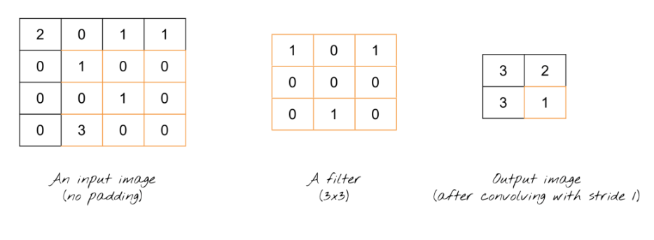
Figure 2: Applying filters in 2D Convolutional Neural Networks. NxN filter is dot-multiplied by NxN portion of the image. This figure illustrates a simple example of an image, a filter, and its corresponding output. (Suhyun, 2019)
Each dot product in a convolution is a scalar that creates a filtered image as output. This image is generated as follows: starting from the top left corner, dot-multiplication is done for every NxN portion of the input image. In Figure 2 the final step is shown: dot-multiplication of the last NxN portion of the image with the filter, resulting in the value of the last element of the output image. The general structure of a CNNs with its distinct layers is visualised in Figure 3.
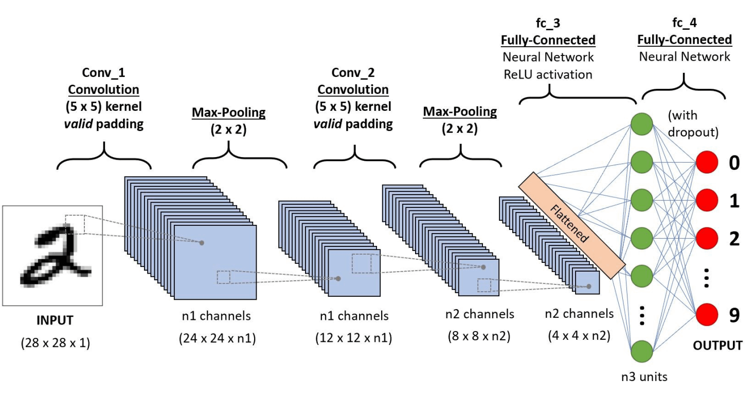
Figure 3: An example of a CNN and its distinct layers. The input is an image. There are multiple concolutional and max pooling layers. The extracted features are flattened before being fed into a classical NN with its respective fully-connected layers. (Saha, 2018).
In a CNN, there are many additional useful layers. These include: pooling layers, fully connected layers, dropout layers, and normalisation layers amongst many others. These layers contribute to increase the efficiency of the image processing. Here are some noteworthy examples: As illustrated in figure 4, Pooling layers are used to progressively reduce the spatial size. They reduce the number of parameters and computations, yet maintain a reasonable accuracy. Another example, are dropout layers. These layers temporarily freeze certain nodes, in an attempt to prevent overtraining. Moreover, the convolutional part of a CNN can also contain normalisation layers in which batch normalisation is performed. These layers adjust and scale the activations to normalise the input layer. In Batch normalisation the node outputs are computed across the predetermined batch and are the same for each example in the batch (Santurkar et al, 2018). Therefore, it is a technique that improves speed, performance, and stability in a CNN (Cooijmans, 2016).
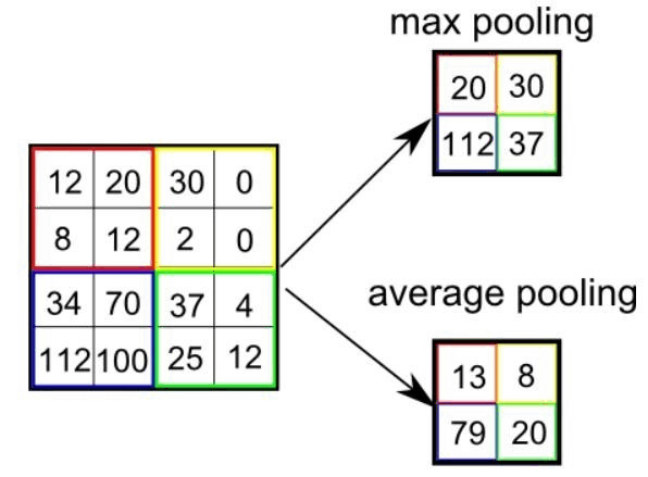
Figure 4: The process of max pooling and average pooling. Pooling is used to diminish the computational requirements yet maintain accuracy. Max pooling takes the highest intensity in an area, average pooling takes the average intensity in an area. (Saha, 2018)
Dual input Convolutional Neural Network
A Dual input Convolutional Neural Network (DiCNN) is a class of NN architectures derived from siamese NNs. They consist of three CNNs built in tandem as illustrated in Figure 5. Two input CNNs each receive an image and extract key features relative to them. These features then get combined into a third CNN. This CNN deconvolutes the information to generate a new image based on the inputs. The aim of deconvolution layers is to reconstruct an image using the features extracted from previous convolution layers. DiCNNs are used to find similarities between inputs and are also useful when attempting to draw a single conclusive output from two separate inputs.
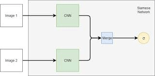
Figure 5: General structure of a DiCNN (Reni, 2019).
Parallax Shift as a Means of Depth Estimation
An efficient way to generate depth estimation is to exploit the binocular disparity of stereo vision. This is the method employed by animal eyes, and can as well be adapted to computer vision. As stereo cameras are horizontally separated, any object in their visual field will be detected along two separate lines of sight. This difference between the cameras results in a phenomenon called parallax, or disparity shift. This phenomenon causes objects to be located in different positions within the two visual frames. The disparity shift is larger for objects that are closer to the cameras, and smaller for objects that are further away. The exact relationship between the disparity shift and the distance to the object is given by the following formula:
z=(f*B)/d
where z is the distance from the camera to the object, d is the disparity shift between the two images, f is the focal length of the camera, and B is the horizontal distance between the camera centers. By training a NN to find similar patterns in an image, the disparity shift could be estimated for subsections of the image. Using this formula, the depth map could then be created (Garg et al, 2016).
Methods
Two methods for depth estimation were designed for stereo vision inputs, which both relied on (C)NNs. Neural Networks were implemented using Pytorch, an open source machine learning library widely praised amongst programmers for its efficiency and ease of implementation. The (C)NNs were built using the structures from the example codes from Reni (2019), Manuel et al, and Whdlgp (2019). The general structure of the CNN was built as a DiCNN (Koch et al, 2015) with the specifics described in Figure 6.
The data used for the training and testing of both NNs was provided courtesy of the University of Tsukuba (UoT, 1997). The dataset was created in 1997 using computer modelling, allowing for the depth maps to accurately represent the depth data of each image.
The dataset is a 60 second video shot at 30fps, totaling 1800 stereo image pairs and their respective depth maps.
Method 1
Structure
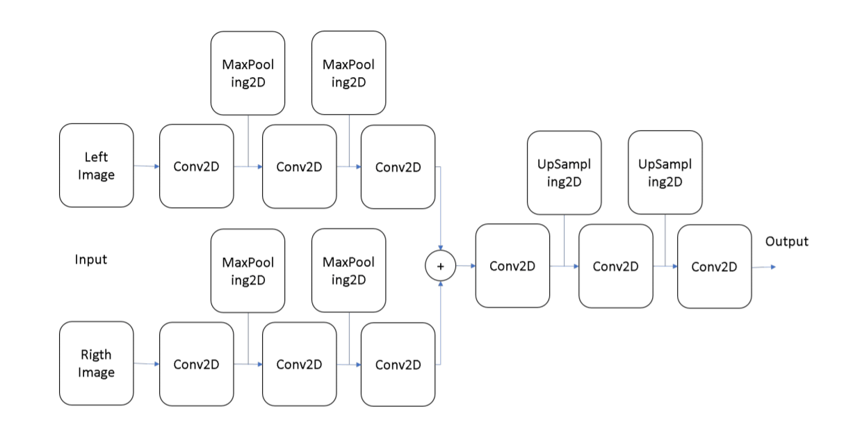
Figure 6: General structure from which is used in the first method where inputs from the left and right images are concatenated at a certain layer (Manuel, et al, 2016).
In order to create a depth map, the first step was to create the structure of the CNN. This consisted of a DiCNN (one for the left and one for the right image), with each input having 3x240x320 nodes, each corresponding to 1 pixel. 240x320 corresponds to the dimensions of the images, and 3 stands for 3 RGB colour channels. Secondly, each of the two inputs reduces the number of nodes, which then combine in the same CNN. During this process, the number of nodes was reduced by the convolutional layers to a number lower than the dimensions of the original image (<240x320). In order to be able to compare the final output, the depth map, the size of information needed to be increased. This was achieved with upsampling. Upsampling added 0 around existing nodes, until the number of nodes reached the required dimensions.
Data Processing
Having the structure of CNN ready, the data needed to be transformed into a suitable form for the CNN training. The images and depth maps were converted into numpy arrays. The images were split into categories based on their illumination conditions and whether they were from the left or right camera. The data was further separated into testing and training data, with 90% of the data as training and the remaining 10% as testing data. The different illumination conditions were of the same 3D environment. As a result, the two depth map files could be used with all sets of camera data, as the depth of the image was independent from the lighting conditions.The final size of the 10 files used for testing was 5.75 GB, whilst the final size of the 10 files used for training was 51.76 GB. This size difference is there since the testing data was 10% of total data. The large file size meant that the size of the dataset fed through the network had to be reduced. Firstly, only the daylight images were chosen, as such lightning conditions seemed the most similar to the lighting conditions faced once the program is used in real life. Only the left depth map dataset was fed to the NN as generating only a single depth map was required to fulfill the aim of this project.
Training of Convolutional Neural Network
The training selection of the images was then fed to the CNN, with left and right versions of the images each fed into their respective input CNN branches. The CNN initially output random depth values for each of the pixels, creating a random depth map. The output was then compared to the real depth map, and the loss evaluated with a binary cross-entropy loss function. Backwards propagation with slow learning rate was then used to slowly adjust the weights and nodes to minimise the loss function and therefore better match the real values. The image feeding process was done for 6 images at a time (batch size), for 40 epochs.Having done the training, the CNN was ready to be tested on a new set of images to evaluate whether it has learned how to create accurate and reliable depth maps.
Method 2
The second method estimated the depth map directly from the disparity shift between left and right images. A Neural Network was designed to predict the similarity of specific portions of the two input images. A comparing function built upon this network was then called for each pixel on the left input image to assess which pixel on the right they best matched. The shift in coordinates between corresponding pixels was then calculated, and from this value the depth was estimated.In addition to Tsukuba dataset, the second method also used a secondary dataset provided courtesy of the Karlsruhe Institute of Technology and Toyota Technological Institute (KITTI, 2012). The latter dataset mainly comprised of stereo images taken from a moving vehicle of city streets. As this dataset did not come with adequate depth data, it was used to test the second method’s ability to perform on unseen data and create disparity maps of new images.
Structure
The structure of the second DiCNN resembled the structure of the first DiCNN. Two stereo image inputs were firstly fed into two convolutional input branches. However, unlike in the first structure, these two inputs were then merged into one non-convolutional NN. The two CNN inputs each consisted of 3x19x19 input nodes, as later on 3x19x19 pixel portions of the image were fed into the CNN. Each of the CNN inputs was then flattened and joint together in the final non-convolutional NN. This last part of the DiCNN reduced the number of nodes to a single output. The output was a value between 0 and 1, corresponding to the similarity between two input images.
Beginning - Minute 5:14
Data Processing
This NN is meant to output a similarity score between 0 and 1 of two images. To that end and to create a suitable dataset, ten images with a large variety of colours and patterns were picked. From each of them, 100 random points were chosen for which pixel portions were created. Then for each of these pixels, a 19x19 portion centred around the chosen pixel was drawn out. This represented the first set of testing images. To create the second set, noise was added to the image. In addition, for every pixel, a new random selection was created with its centre positioned randomly up to ± 19 pixels on the x-axis and ± 19 pixels on the y-axis. This process resulted in pixel selection pairs. As the location of these pairs was known, the similarity score was evaluated with the overlap amount, as illustrated in Figure 7. In other words, two selections fully overlapping would score a 1 and two selections 19 pixels away from each other would score a 0. This process produced 10 datasets, each with an array for the original image pixel selections, an array for the noisy image shifted pixel selections, and 100 corresponding similarity scores.
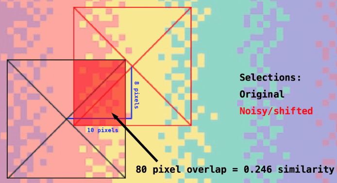
Figure 7: Shift of 10 and 8 pixels on a 19x19 selection showing original and shifted area selections for NN training.
Training of the Neural Network
Before providing the NN with real data, it had to be trained on how to recognise the similarity between two input images. That was done by inputting a 19x19 selection of an image into one of the two CNN input channels and its slightly shifted and noisy version in the second input CNN channel. The Neural Network would then output a value (0-1) for the similarity between the two sections of the image. The similarity value that the NN predicted was compared to the actual similarity value. Backwards propagation was then used to adjust weights and nodes in order to minimise the loss function, which gave the difference between the actual similarity and the one predicted by the NN. Both of the CNN input branches’ weights and nodes were adjusted independently of one another. Backwards propagation was used until the loss function approached zero, while the order in which the selection pairs and their similarities were loaded was shuffled to minimise the possibility of the NN picking up on unintended patterns and not learning the correct relationship between the depth and disparity.
Iteration algorithm
The first step of the iteration algorithm was to determine the disparity shift of every pixel by comparing portions of the two images via the Neural Network. For each pixel on the left stereo image, a 19x19 window was created around it. At the same time, a window of the same size was also created around the pixel with the same coordinates on the right image. A compare function, built upon the NN, was responsible for assessing the similarity of the two windows. From this similarity, a score ranging from 0 to 1 was assigned to the pixel in the center of the right window using the NN. Then the right window was shifted along the horizontal axis in steps of one pixel, and each time the compare function was called to compare the new windows on the right with the original one on the left. This iteration occurred only for a specific region of the right image, referred to as the search area, chosen to be 20 pixels for the x coordinates and 2 pixels for the y coordinates.
For any given pixel on the left image, the pixel with the highest similarity score on the right search area was selected to be the corresponding element. A disparity value was then calculated from the difference in the coordinates of the two analogous pixels, and this value was then assigned to the original pixel on the left image.
The process is iterated throughout every pixel in the left image so that the final output was one picture filled with disparity values. If the pixel in question was located near the edges of the images, the window would extend to a field of newly-created, padded pixels with value -1, so that the compare function would not account for them.
The final step of the algorithm was to determine the depth from the disparity values. The depth was calculated based on the disparity shift formula. The depth then had to be normalised. This was done by selecting the maximum and minimum calculated depth values, and normalising all values to a new range whose bounds were determined by the maximum and minimum values. The new range was chosen to be from 0 to 255 m away from the camera.
The second method is heavily limited by the predefined search area surrounding the selected pixel. For situations in which objects are so close to the camera that they may not appear on both stereo images, or where they both appear but are outside the bounds of the search area, this method is not applicable. To avoid this limitation, the code would have to search the whole image for a potential match, greatly increasing processing power and time required.
Implementation of StereoPi
To be able to create depth maps in real-time, the project needed a stereoscopic camera. A relatively cheap and practical solution was to use a StereoPi device. This is a modified Raspberry Pi (a small GNU/Linux computer) that includes two PiCamera sockets and as such allows its use for stereo imaging. The StereoPi came without any useful mounting support for this projects purposes, therefore a housing was designed using a CAD software which was then 3D printed (see Figure 8 for the assembled PyDepth project camera).
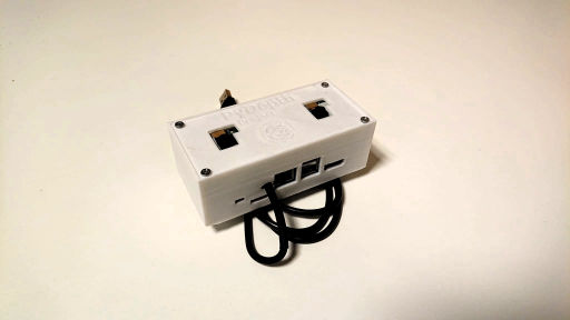
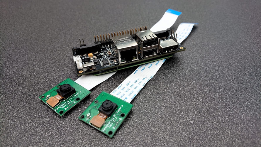
Figure 8: Assembled PyDepth project camera (left) and internal components (right).
Given the relatively small computing power of the Raspberry Pi, it was decided that instead of running the NN on the Raspberry Pi, the video would be streamed through a local network onto another computer with greater processing power. This computer would then run the NN and compute depth maps. The connection was made using Python sockets that create a client-server tunnel between the two devices. The images were transformed into a byte stream and sent from the StereoPi (client) towards the main computer (server) and reconstructed using OpenCV to create the live feed. Every tenth frame was saved into an external data files as numpy arrays to be fed into the Neural Networks. The software written can be used on Linux, Windows and MacOS computers.
Results and Discussion Method 1
In the training phase, this method initially gave very promising results, but it quickly became clear that the network was only overtraining on the given data-set. This was evident from the features as they seemed to be too specific. This was then confirmed by feeding in the testing data-set which only contained pictures that had never been given to the network. The resulting depth maps were extremely inaccurate, as can be seen by comparing Figure 9a, which displays the overtrained network output, and Figure 9b, showing the inaccurate output on testing data.
The output seen in Figure 9a has specific features, mainly the shadows outlining the shapes. These specifics support the idea of overtraining that was probably caused by the nature of the dataset: the dataset was made up of frames extracted from a video. This meant that many of the frames had very similar features which, as a result, trained the network in a very narrow and specific way. This in turn had an impact on the processing of the new dataset, as seen in Figure 9b, as the network was not able to recognise the features it had learned by heart. As a result the output of the network were inaccurate depth maps.
To solve the overtraining issue, the dataset was expanded upon by flipping the images in three different ways: flipping over the x-axis only, over the y-axis only, and over both the x and y axes. This was done in order to diversify the dataset to make the features that the network previously overtrained on less accessible. This solution did not work as intended as it did not stop the network from overtraining.
Other methods to prevent overtraining were considered, but due to time constraints, they were not applied in this project. Firstly, a more diverse dataset could have been implemented, which would have given the neural network a higher diversity of inputs. This would have mitigated the issues presented by the similarity of the video frame dataset and provided a more effective NN. Another possibility would have been to simplify the network architecture. Complex networks present the possibility of overfitting, in which the network has too many free parameters, and as a result, can begin to memorise features. An attempt was made to simplify the network, but the extended training time combined with no major improvements being observed in the initial stages of training led to this method being abandoned. Given more time, different structures and architectures could have been tried, possibly improving the outcome of our NN. Another technique, called regularisation, could have been implemented. In this case in the form of weight decay, this technique lets all parameters of the model slowly approach zero unless relevant for the prediction in order to reduce their freedom. As a result, the model would have been less likely to fit noise and thus less likely to overfit. One last possible addition could have been the use of dropout layers which are specifically designed to reduce overfitting. They perform model averaging efficiently and thus simplify the NN.
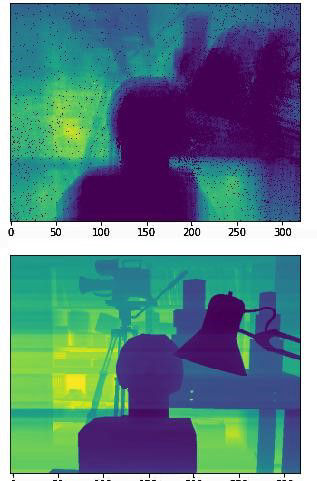
Figure 9a: Training outputs from the training data after 40 epochs from the first method. specific features can be seen due to shapes outlined by shadows.
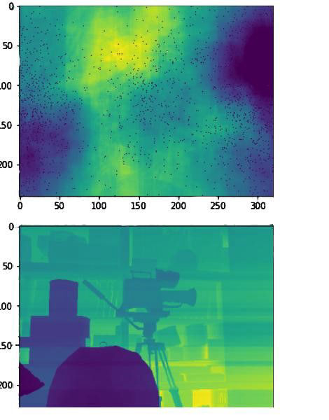
Figure 9b: Figure 9b: Results from the test data from the first method (same network).
Results and Discussion Method 2
Minute 5:14-End
The issues encountered in the first method were mitigated in the second by replacing parts of the network with an iteration algorithm. Different datasets were used to train the Neural Network which yielded various results discussed below. To compare the performance of the different networks and to check the correctness of the algorithm, the image pair shown in Figure 10 was used as a testing image.
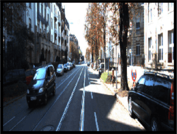
Figure 10: Left Test Stereo Image (KITTI dataset)

Figure 10: Right Test Stereo Image (KITTI dataset)
Figure 11 showcases one of the first depth maps that were generated using the second method which could indicate a faulty algorithm and/or a poorly trained network. When overlaid with the original image, as displayed in Figure 12, it is visible that the network specifically detects edges.
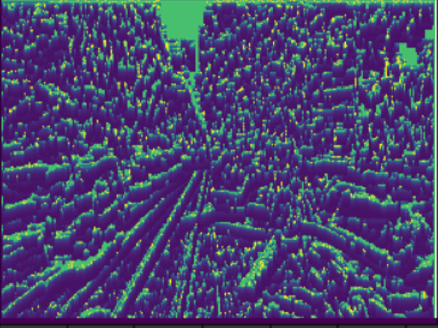
Figure 11: Example of a (attempted) generated disparity map using the second method on the images from Figure 10. Green pixels are meant to show large disparities whereas dark blue pixels should show small disparities.
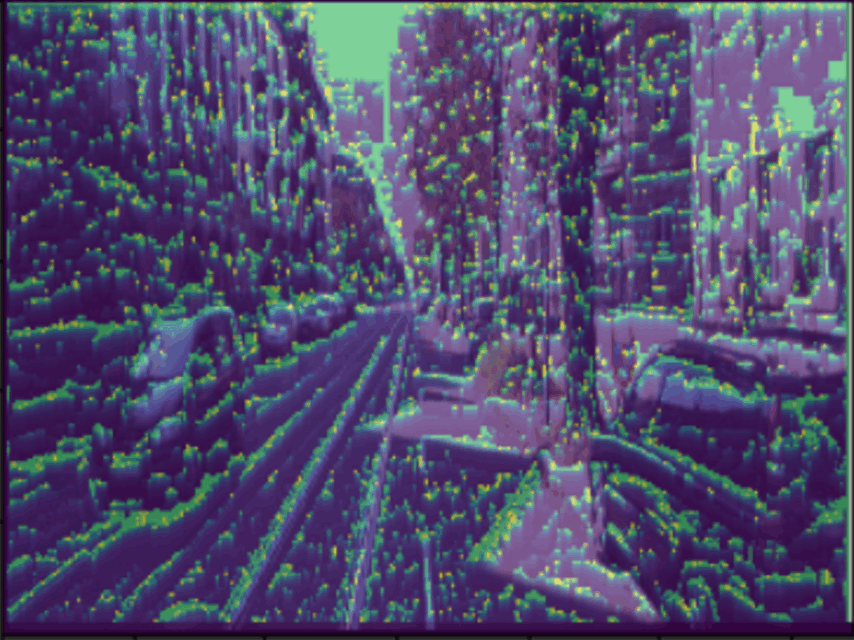
Figure 12: Overlay of the image and its corresponding depth map from figure 11. This figure shows that the edges that seem to appear in figure 11 do overlap with the original image, implying a form of edge detection.
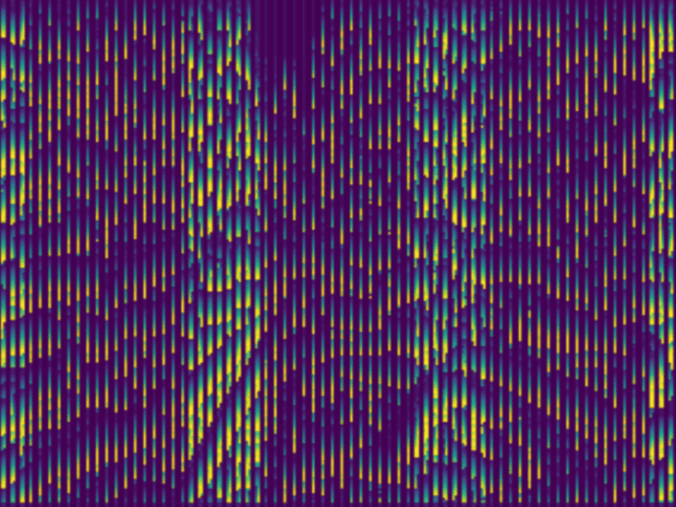
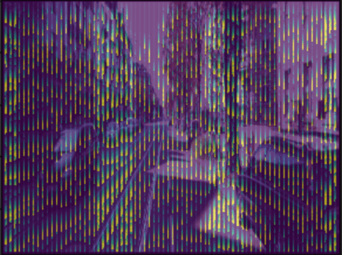
After the first attempts, the generated depth maps always followed a specific pattern where bright pixels were followed by a vertical gradient (Figure 13). This was much more visible after the search area was increased for computational purposes (leading to thicker and more visible stripes) and could indicate that instead of iterating horizontally, the pixels were compared vertically. Therefore, the results were unclear as theoretically there should not be any disparity shifts in the vertical direction. This could also account for the NN returning an edge detection that only works for non-vertical edges: on a vertical edge, all pixels look the same as seen from a small enough area whereas a diagonal or horizontal edge would have different pixels when looked at horizontally.
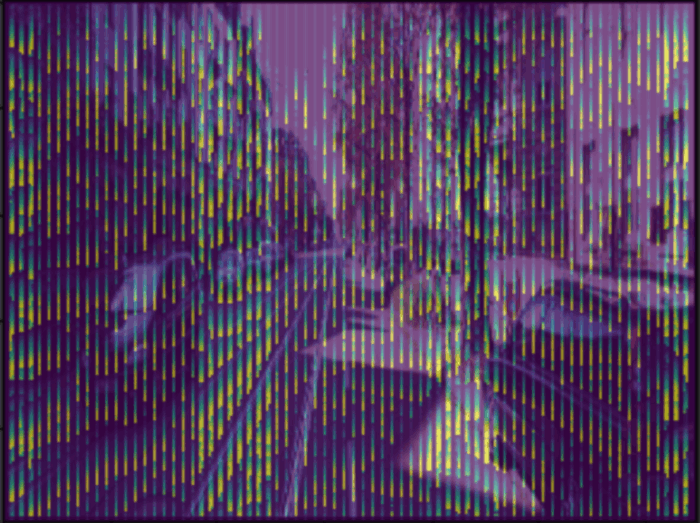

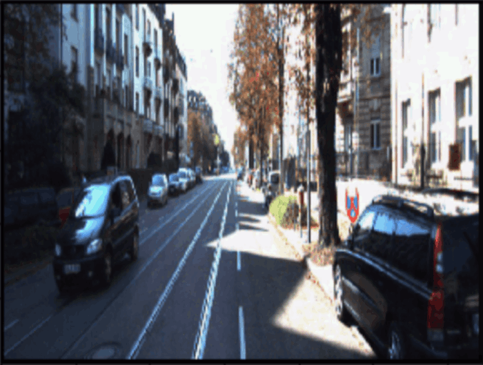
Figure 13: Three figures to illustrate the disparity maps relative to the vertical ittertations. (Right) Testing image. (Centre) Predicted disparity map. (Left) Overlay of both right and centred images.
Subsequently, the vertical iteration issues in the outputs were resolved by rewriting the iterative algorithm. Unfortunately, this pattern persisted and was observed horizontally. It was apparent that the network was regrettably only detecting edges instead of depths (Figure 13).
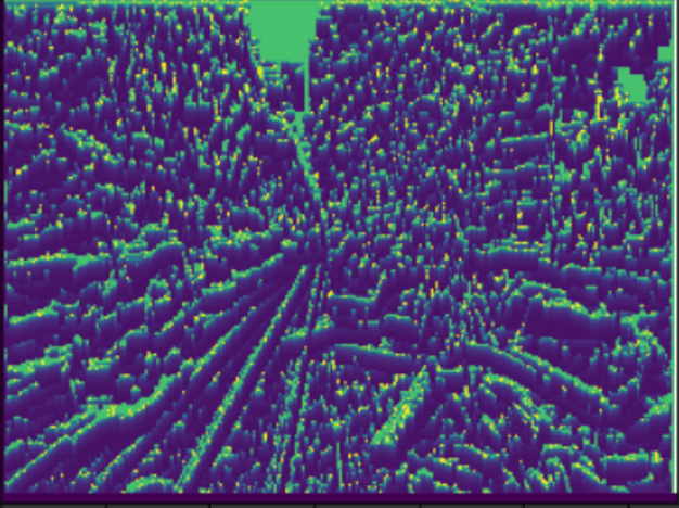
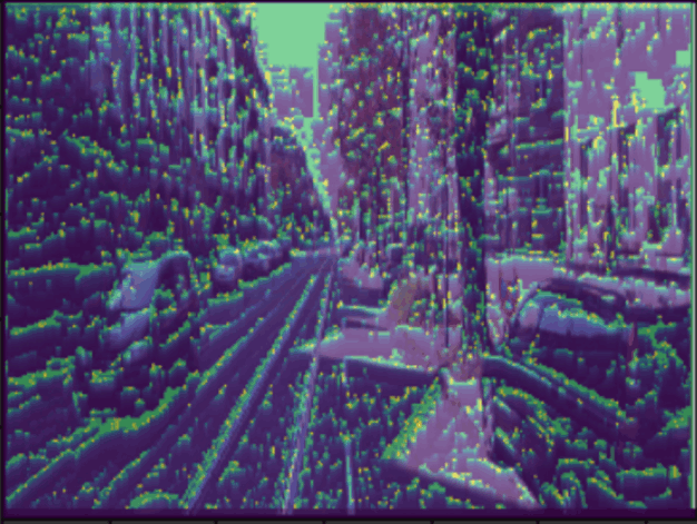
The observed ‘streaks’ were assumed to be a result of a specific malfunction of the neural network: it seemed as though there were certain pixels that were assigned a very high similarity score independently from the pixels they were compared with. This could indicate that one pixel (e.g. pixel 10/20 on the right image) would obtain a very high similarity score with all the pixels from the left image - meaning that 10/20, 11/20, 12/20 … 30/20 (up until 10/20 is outside of the search area, in this case, a search area of width 20) would all be matched up with 10/20 from the right image. Since the distance was found based on the pixel shift, and the program iterates through the image, the assigned distance values would gradually increase as the pixel shift was changing. This resulted in the fading ‘streaks’ seen in Figure 14.
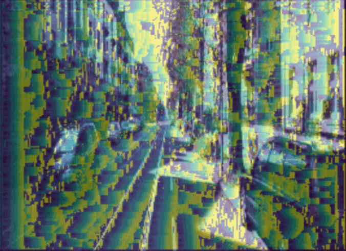
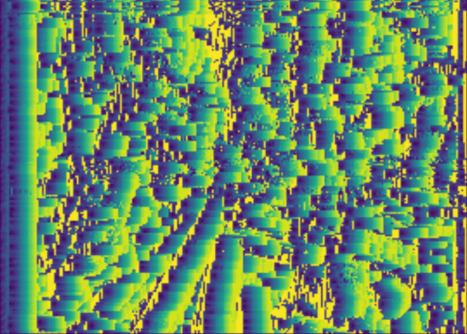
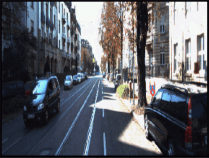
Figure 14: Three figures to illustrate the disparity maps relative to the horizontal iteration. (Right) Testing image. (Centre) Predicted disparity map. (Left) An overlay of the two other pictures to underline similarities and differences.
A solution to this problem has yet to be found, as all the attempted approaches, including those described in the First Method Results and Discussion, yielded no conclusive results. The only pattern that was recognised was that pixels near object edges seemed to trigger this problem, hence leading to a result that looked like edge detection.
The current method took a pixel from the left image and iterated over n pixels on the right image to compare the similarity scores. It then chose the right pixel with the highest similarity. This procedure is represented by the graph in Figure 15. In this graph, the x-axis represents how far the pixels on the right image have been checked relative to the pixel from the left image. The y-axis shows the output of the Neural Network for a specific pixel and in this particular example, the correct pixel shift is 10. If the images overlap perfectly (at a shift of 10) the NN is expected to output a 1, while as the selection moves away from the perfect overlap the similarity should decrease until (for a 9x9 window) it reaches a value of 0 overlap at shift <1 and >19. This is illustrated as the black dotted line in Figure 15.
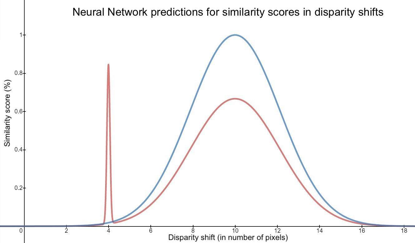
Figure 15: Graph explaining why certain pixels are always seen as more similar due to them being outliers. On the x-axis, we have the amount of disparity shift in pixels on the y-axis, we have the similarity score predicted by the neural network in percent.
In reality, what actually seemed to occur, was that the NN would make periodic mistakes. The red line in Figure 15 shows what would take place if the NN predicted a perfect overlap in a random wrong position. With a spike, the highest similarity score would replace the real maximal shift and lead to a faulty result. Even with idealistically near-perfect accuracy of 99%, as every pixel is compared to about 90 other pixels from the right image, it would still result in about half of all pixels being assigned the wrong similarity score.
In order to fix the issue, a smoothing function was essential. The area under the curve (AUC) or integral was used. The regions of similar pixels selections were evaluated by checking which region had the highest AUC. In doing so, these inevitable artifacts were eliminated. As illustrated in Figure 15, even though f(4)has the highest similarity score, the adjacent pixels have a rather low similarity score in comparison. In this case, f(10)with its similarly high valued surrounding pixels, it would have been chosen as the best-matched location.
Whilst this alteration did lead to smaller ‘streaks’ (Figure 16) compared to the method without the AUC technique (Figure 13), it did not fully resolve the issue. The iterative algorithm was further tested with random similarity scores that demonstrated that the ‘streaks’ were not caused by the algorithm. As such, it was thought that the main issues lie with the network.
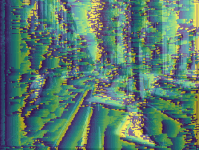
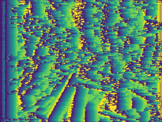
Figure 16: Three figures to illustrate the disparity maps relative to the horizontal iteration after using a smoothing function. (Right) Testing image. (Center) Predicted disparity map. (Left) Overlay of both right and centred images.
In an attempt to fix this issue, the NN was trained to be image specific. This meant that instead of training it on various datasets of pixel selections, it was instead trained specifically on the two images that were evaluated. With this approach, it was hypothesised that the network would be able to pick up on image-specific patterns and therefore perform better. Despite these efforts, the results were at this point only random patterns.
There were numerous hypotheses as to why the Neural Network might not have been performing up to standards. Indeed, only training the data on two images would not generate sufficient training data to achieve pattern recognition. Instead, other machine learning techniques could have been better suited in these conditions. Some possible considerations could have been: Random Forest, Restricted Boltzmann Machines, and Support Vector Machines.
Ideally, a fully tailored implementation would have been necessary, which while certainly possible, would have been highly improbable due to the time constraints.
In addition to the above-described problems, there was also the possibility that some sources of errors lie in the dataset that was used for training. Indeed, in order to prevent the network from simply comparing exact pixel values, some levels of random noise were added to the training process to simulate slight differences between the two cameras. As such, it may well be that this artificial random noise was not a good representation of natural divergences in the properties of the cameras.
Conclusion
The goal of this project was to recreate accurate depth maps given stereo images. Two main approaches were explored, with a possibility to combine their results in the end. Both methods ran into unexpected issues which, due to time constraints, were not completely resolved and led to inconclusive results.
The first approach employed a Dual input Convolutional Neural Network built using PyTorch and based on an already existing model (Whdlgp, 2019). The network was supposed to independently learn features from stereo images and recognise the disparities as features to build depth maps. This method did not yield very promising results due to overtraining. Several attempts were made to resolve the issue, such as extending the dataset and simplifying the network. However, no major improvements were observed. Given more time, several other attempts could have been carried out to prevent overfitting, such as further simplifying the architecture, increasing the diversity of the dataset, implementing regularisation, or adding dropout layers.
The second method combined both iteration algorithms and neural networks. Instead of adopting a big NN for all feature recognition, a smaller NN was used only for the recognition of similar pixels. The disparities between the two images were then mapped by the iteration algorithm. Based on the disparity, the depth was calculated. The issue with this method seemed to have been the inaccurate predictions by the NN. For some pixels, the NN seemed to have assigned high similarity values to multiple pixels, resulting in streaks. As high similarity pixels were usually the edges, the algorithm appeared to act as an edge detector. Multiple approaches were adopted in an attempt to fix the problem, but none were fruitful.
Using a StereoPi outfitted with two stereo cameras, and mounted in a bespoke 3D printed housing case, a previously trained network (Pomazov, 2019) could be implemented, which successfully created real-time depth maps in video format. This showed that should the NN be functional, the goal of the project would have indeed been achieved.
Despite the project not offering ideal results, the StereoPi shows that the end goal is achievable and that the presented hardware is sufficient. Given more time, some improvements could still be done to fix the existing issues. The long computation times prohibited in the implementation of solutions and hence not all proposed approaches could have been implemented. Future work on this project should focus on implementing these approaches, which are expected to further the progress of the current results. That would eventually lead to a functioning PyDepth module which could then be implemented in different situations like object avoidance or scene reconstruction.
References
Cooijmans, T., Ballas, N., Laurent, C., Gülçehre, Ç., & Courville, A. (2016). Recurrent batch normalization. arXiv preprint arXiv:1603.09025. https://arxiv.org/pdf/1603.09025.pdf
Fonau, S. Z., Javar, T., Lemoine, S., McKiernan, F., Quinque, F. (2019). PyStalk https://hollyqui.github.io/PyStalk.html
Garg, R., BG, V. K., Carneiro, G., & Reid, I. (2016, October). Unsupervised CNN for single view depth estimation: Geometry to the rescue. In European Conference on Computer Vision (pp. 740-756). Springer, Cham. https://arxiv.org/pdf/1603.04992.pdf
Haykin, S. S. (2009). Neural networks and learning machines/Simon Haykin. Retrieved from: (PDF) Neural Networks and Learning Machines 3rd Edition | Duc Nguyen
Hecht-Nielsen, R. (1992). Theory of the backpropagation neural network. In Neural networks for perception (pp. 65-93). Academic Press. http://www.andrew.cmu.edu/user/nwolfe/esr/pdf/backprop.pdf
KITTI Stereo Evaluation Dataset retrieved from: http://www.cvlibs.net/datasets/kitti/eval_stereo_flow.php?benchmark=stereo
Koch, G., Zemel, R., & Salakhutdinov, R. (2015, July). Siamese neural networks for one-shot image recognition. In ICML deep learning workshop (Vol. 2). http://www.cs.toronto.edu/~gkoch/files/msc-thesis.pdf
Lawrence, S., Tsoi, A. C., & Back, A. D. (1996). Function approximation with neural networks and local methods: Bias, variance and smoothness. In Australian conference on neural networks (Vol. 1621). Australian National University. http://machine-learning.martinsewell.com/ann/LaTB96.pdf
Manuel, M. G. V., Manuel, M. M. J., Edith, M. M. N., Ivone, R. A. P., & Ramırez, S. Disparity map estimation with deep learning in stereo vision. http://klab.uacj.mx/rccs/2018/post/00030027.pdf
Pomazov, E. (2019). OpenCV and Depth Map on StereoPi tutorial. Retrieved from : https://medium.com/stereopi/opencv-and-depth-map-on-stereopi-tutorial-62cb6792bbed
Reni, R. (2019, January 28). Siamese Neural Network with Pytorch. Retrieved from https://innovationincubator.com/siamese-neural-network-with-pytorch-code-example/
Saha, S. (2018, December 15). A Comprehensive Guide to Convolutional Neural Networks — the ELI5 way. Retrieved from: https://towardsdatascience.com/
Santurkar, S., Tsipras, D., Ilyas, A., & Madry, A. (2018). How does batch normalization help optimization?. In Advances in Neural Information Processing Systems (pp. 2483-2493). https://papers.nips.cc/paper/7515-how-does-batch-normalization-help-optimization.pdf
Suhyun, K. (2019). A Beginner’s guide to Convolutional Neural Networks (CNN). Retrieved from: https://towardsdatascience.com/a-beginners-guide-to-convolutional-neural-networks-cnns-14649dbddce8
University of Tsukuba Stereo Image Dataset retrieved from: https://home.cvlab.cs.tsukuba.ac.jp/dataset
Venturelli, M., Borghi, G., Vezzani, R., & Cucchiara, R. (2017). From depth data to head pose estimation: a siamese approach. arXiv preprint arXiv:1703.03624.
Whdlgp. (2019). Disparity estimation with keras. Retrieved from https://github.com/whdlgp/keras_cnn_disparity
Xu, D., Wang, W., Tang, H., Liu, H., Sebe, N., & Ricci, E. (2018). Structured attention guided convolutional neural fields for monocular depth estimation. In Proceedings of the IEEE Conference on Computer Vision and Pattern Recognition (pp. 3917-3925). http://openaccess.thecvf.com/content_cvpr_2018/papers/Xu_Structured_Attention_Guided_CVPR_2018_paper.pdf
Appendix
| What | Who |
|---|---|
| Abstract | Timour |
| Introduction | Jonas, Alica, Leonoor, Timour, Giovanni |
| Methods | Alica, Leonoor, Marco, Giovanni, Timour, Jonas |
| Results and Discussion | Syzmon, Felix |
| Video | Syzmon, Felix |
| Conclusion | Syzmon, Felix |
| Reviewing | Everyone |
| Editing for Structure and Coherence | Timour, Leonoor, Marco, Giovanni, Alica, Jonas |
| Website | Alica |
| NAME | ID | @ |
|---|---|---|
| Felix Quinque | i6166368 | f.quinque@student.maastrichtuniversity.nl |
| Szymon Fonau | i6161129 | s.fonau@student.maastrichtuniversity.nl |
| Leonoor Verbaan | i6165892 | l.verbaan@student.maastrichtuniversity.nl |
| Timour Javar Magnier | i6175968 | t.javarmagnier@student.maastrichtuniversity.nl |
| Jonas Tjepkema | i6194103 | jpm.tjepkema@student.maastrichtuniversity.nl |
| Giovanni Rupnik Boero | i6089271 | g.rupnikboero@student.maastrichtuniversity.nl |
| Alica Rogelj | i6192517 | a.rogelj@student.maastrichtuniversity.nl |
| Marco Fiorito | i6186083 | m.fiorito@student.maastrichtuniversity.nl |